Working faster in Excel
We all like to save time by using Excel. However, when working on large spreadsheets, it’s easy to get lost on what data is in which column.
Here’s a tip from our client David Ringstrom that will help you keep track of where all your data is on a large spreadsheet.
by Guest Editor David Ringstrom with Accounting Advisors
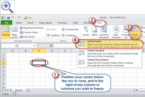
Freezing or unfreezing worksheet panes typically involves multiple mouse clicks, but I’ll show you a way to carry out this task with a single keystroke. For the uninitiated, freezing panes allows you to lock in place columns or rows that you specify along the left-hand and/or top of Excel’s worksheet area. As you scroll to the right or down, the frozen columns or rows remain in place so that you can always view worksheet headings or the initial columns. When you no longer need the rows or columns locked in place, you, in turn, can unfreeze them.
Figure 1: An example of freezing panes on a worksheet.
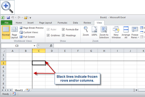
Figure 2: Thin black lines indicate frozen rows and/or columns.
As shown below, a thin black bar appears below a set of frozen rows, and to the right of any frozen columns. To unlock the rows or columns, navigate to the View tab, choose Freeze Panes, and then Unfreeze Panes. It’s a little simpler in Excel 2003: choose Window, and then Freeze Panes or Window, and then Unfreeze Panes, respectively.
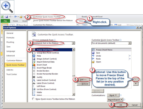
Regardless, you streamline this process down to a simple keystroke of your choice in Excel 2007 and later. To do so, as shown in Figure 3, right-click on the View tab in Excel, and then choose Customize Quick Access Toolbar to display the Excel options window. Select Commands Not in the Ribbon, and then scroll down the resulting list until you find Freeze Sheet Panes. Either double-click on this command, or click once on it and click Add to add it to your Quick Access Toolbar. If you frequently freeze and unfreeze sheet panes, use the arrows on the right-hand side to move the Freeze Sheet Panes command so that it’s the first command on the list. Click OK to close the Excel Options dialog box.
Figure 3: Add Freeze Sheet Panes to your Quick Access Toolbar
Once you’ve placed the command on your Quick Access Toolbar, you can now press the Alt key to reveal the numeric shortcut for the Freeze Sheet Panes command. If you made it the first command on the list, you can now press Alt-1 to freeze or unfreeze sheet panes. You must still position your cursor as before when freezing panes, but you can bypass navigating through the View tab and the resulting Freeze Panes submenu.
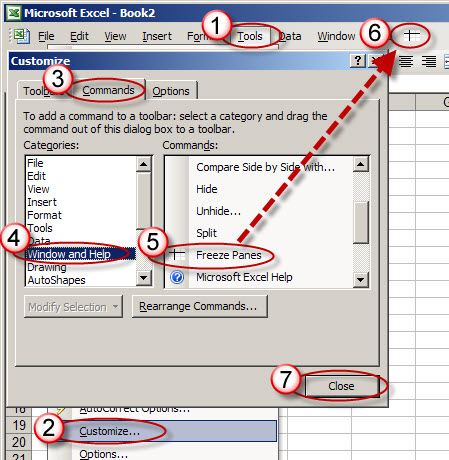
Excel 2003 users can also give themselves one-click access to freezing/unfreezing panes, sans keyboard shortcut. As shown in Figure 4, choose Tools, Customize, and then click on the Commands tab. Choose Window, and then drag the Freeze Panes command either onto an existing toolbar or to Excel’s menu bar, into the unused space adjacent to the Help menu.

Figure 4: Excel 2003 users can arrange one-click access to the Freeze Panes command.


